TOVsolver module guide

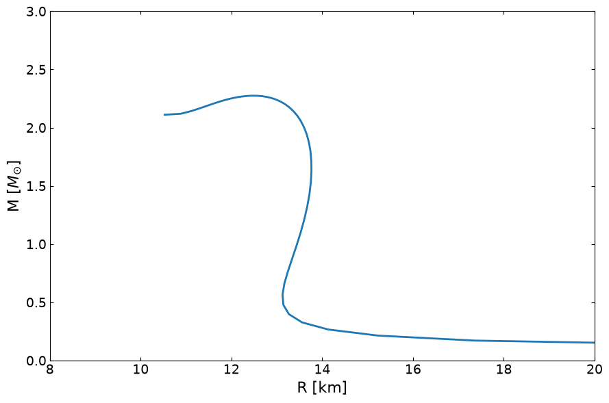
TOV solver part we have multiple function, we can generate a Mass radius function from ‘Test_EOS.csv’ file here easily

from pathlib import Path
import sys


def find_repo_root(start=Path.cwd()):
    for path in (start, *start.parents):
        if (path / "pyproject.toml").exists():
            return path
    return start


NOTEBOOK_DIR = Path.cwd()
REPO_ROOT = find_repo_root(NOTEBOOK_DIR)
if str(REPO_ROOT) not in sys.path:
    sys.path.insert(0, str(REPO_ROOT))

import matplotlib.pyplot as plt
import TOVsolver.main as main
from TOVsolver.unit import km, Msun


def find_test_eos():
    candidates = [
        NOTEBOOK_DIR / "Test_EOS.csv",
        NOTEBOOK_DIR / "Test_Case" / "Test_EOS.csv",
        REPO_ROOT / "Test_Case" / "Test_EOS.csv",
    ]
    checked = []
    for candidate in candidates:
        candidate = candidate.resolve()
        if candidate in checked:
            continue
        checked.append(candidate)
        if candidate.exists():
            return candidate
    paths = ", ".join(str(path) for path in checked)
    raise FileNotFoundError(f"Could not find Test_EOS.csv. Checked: {paths}")


TEST_EOS_PATH = find_test_eos()

# Main has two functions
#   OutputMR() returns mass and radius
#   OutputMRT() returns radius, mass, and tidal deformability
#   OutputC_s() returns the speed of sound and density grid
# The input can be either a CSV path or density/pressure arrays.
MR = main.OutputMR(str(TEST_EOS_PATH)).T

fig, ax = plt.subplots(1, 1, figsize=(9, 6))
ax.plot(MR[1] / km, MR[0] / Msun, lw=2)
ax.set_ylabel(r"M [$M_{\odot}$]", fontsize=16)
ax.set_xlabel("R [km]", fontsize=16)
ax.set_xlim(8.0, 20.0)
ax.set_ylim(0, 3)
ax.tick_params(top=1, right=1, which="both", direction="in", labelsize=14)
ax.tick_params(top=1, right=1, which="both", direction="in", labelsize=14)
fig.tight_layout()
plt.show()

/opt/hostedtoolcache/Python/3.11.15/x64/lib/python3.11/site-packages/scipy/integrate/_ode.py:418: UserWarning: dopri5: step size becomes too small
  self._y, self.t = mth(self.f, self.jac or (lambda: None),

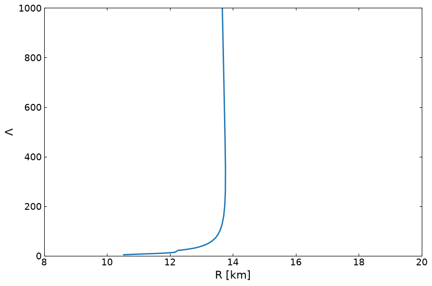
We can generate the tidal property from it also,like tidal deformability

# Try solving the tidal property.
MRT = main.OutputMRT(str(TEST_EOS_PATH)).T

fig, ax = plt.subplots(1, 1, figsize=(9, 6))
ax.plot(MRT[0] / km, MRT[2], lw=2)
ax.set_ylabel(r"$\Lambda$", fontsize=16)
ax.set_xlabel("R [km]", fontsize=16)
ax.set_xlim(8.0, 20.0)
ax.set_ylim(0, 1000)
ax.tick_params(top=1, right=1, which="both", direction="in", labelsize=14)
ax.tick_params(top=1, right=1, which="both", direction="in", labelsize=14)
fig.tight_layout()
plt.show()

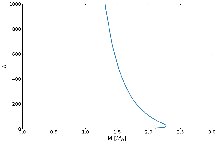
Plot out Tidal with mass

fig, ax = plt.subplots(1, 1, figsize=(9, 6))
ax.plot(MRT[1] / Msun, MRT[2], lw=2)
ax.set_ylabel(r"$\Lambda$", fontsize=16)
ax.set_xlabel(r"M [$M_{\odot}$]", fontsize=16)
ax.set_xlim(0.0, 3.0)
ax.set_ylim(0, 1000)
ax.tick_params(top=1, right=1, which="both", direction="in", labelsize=14)
ax.tick_params(top=1, right=1, which="both", direction="in", labelsize=14)
fig.tight_layout()
plt.show()

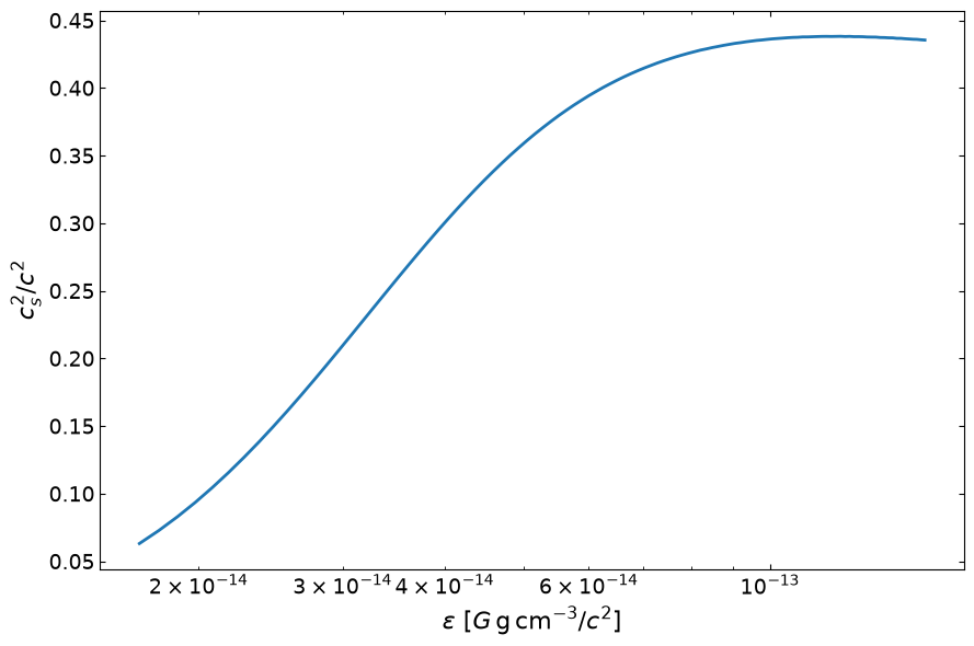
Can generate the speed of sound from the given equation of state. This do not need to solve TOV equation, the speed of sound is defined by the derivative of P(rho) curve, this quantity is very of interest, since whether there is a upper limit of this speed of sound (except for the casaulity limit c_s < 1 ) is a very interesting and hot topic

# OutputC_s returns c_s^2/c^2 and the geometrized energy-density grid.
C_s, rho = main.OutputC_s(str(TEST_EOS_PATH))

fig, ax = plt.subplots(1, 1, figsize=(9, 6))
ax.plot(rho, C_s, lw=2)
ax.set_xlabel(r"$\epsilon$ [$G\,\mathrm{g\,cm^{-3}}/c^2$]", fontsize=16)
ax.set_ylabel(r"$c_s^2/c^2$", fontsize=16)
plt.xscale("log")
ax.tick_params(top=1, right=1, which="both", direction="in", labelsize=14)
ax.tick_params(top=1, right=1, which="both", direction="in", labelsize=14)
fig.tight_layout()
plt.show()

This package can easily integrated into a Baysian inference flow, to do bayesian inference, Here, we generated several (50) EoSs from RMF model, and try to use a loop to compute out all of their MRT property. That could be a in-between step of doing bayesian inference of neutron star EoS. Remember these EoS could also be polytrope, or anything that generate from your own EoS computation code. Next step for us will be integrate our EoS computation into this package and also the Bayesian analysis.